Univariate Probability Spaces
Discrete Domains & Distributions
Definition
Let us create a probability distribution of an experiment that simulates a die. In order to do so, we create a subtype of the jpt.distributions.univariate.Integer class with the range of values that is typical to a fair dice, namely \(\{1, ..., 6\}\):
[24]:
import numpy as np

from jpt.distributions import IntegerType

Die = IntegerType('Die', lmin=1, lmax=6)
Die
[24]:
jpt.distributions.univariate.Die
jpt.distributions.IntegerType is function that dynamically creates a subclass of Integer with the passed string as its name and configures it with the respective range of integer values given by its lower and upper bounds passed as lmin and lmax arguments, respectively.
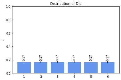
We can create a specific distribution over these possible outcomes of a toss by instantiating the newly created class and setting the parameters of the distribution object. For example, we create the distribution of a fair dice by assigning all values the uniform distribution and plot it in diagram:
[25]:
fair_die = Die()
fair_die.set([1 / 6] * 6)
fair_die.plot(view=True)
We can also compute the moments of the distribution like expectation and variance:
[26]:
fair_die.expectation()
[26]:
3.5
[27]:
fair_die.variance()
[27]:
2.9166666666666665
We can query for the probability of specific events, e.g. the probability that the result of a dice will be 1,
[28]:
fair_die.p(1)
[28]:
0.16666666666666666
or that the result will be greater than 3
[29]:
fair_die.p({4, 5, 6})
[29]:
0.5
The most probable events can be obtained from
[30]:
fair_die.mpe()
[30]:
(0.16666666666666666, {1, 2, 3, 4, 5, 6})
which are, of course, all values in the uniform distribution at hand.
Manipulating Distributions
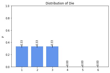
We can manipulate an integer distribution by “cropping” it to a selection of allowed values. All other value will be assigned 0 probability and the remaining values’ probability mass gets adjusted proportionally:
[31]:
biased_dice = fair_die.crop({1, 2, 3})
biased_dice.plot(view=True)
Note that the original distribution has remained untouched by this operation:
[32]:
fair_die
[32]:
<Die p=[1: 0.167; 2: 0.167; 3: 0.167; 4: 0.167; 5: 0.167; 6: 0.167]>
Learning Distributions from Data
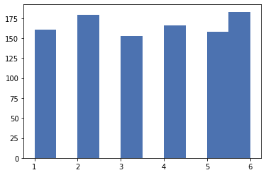
We can use the instantiated object for conducting experiments with the distribution using its sample() method:
[33]:
from matplotlib import pyplot as plt
data = list(fair_die.sample(1000))
plt.hist(data)
plt.show()
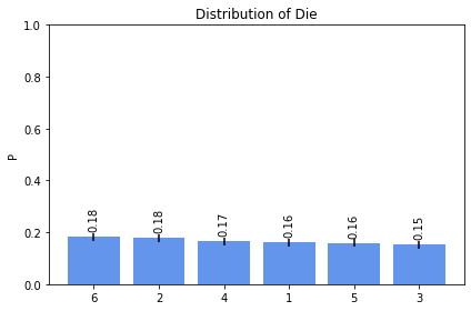
The parameters of a distribution can be learnt from data using its fit() method:
[34]:
learnt_die = Die()
learnt_die.fit(np.array(data))
learnt_die.plot(view=True)
Continuous Domains & Distributions
The pyjpt package provides means for representing and acquiring probabilty distributions of any arbitrary shape over continuous variable domains. As the probability of an event is defined as the area under the probability density function (PDF), single scalar values of variables have 0 probability mass in continuous probability spaces. Therefore, events with non-zero probability must be specified by means of intervals, i.e. continuous sets in \(\mathds{R}\).
Real-valued Sets
pyjpt implements real-valued interval calculus in the jpt.base.intervals package. Intervals can be represented by instances of the jpt.base.intervals.ContinuousSet class:
[35]:
from jpt.base.intervals import ContinuousSet
i1 = ContinuousSet(0, 1)
i2 = ContinuousSet.parse(']2,inf[')
i1, i2
[35]:
(<ContinuousSet=[0.000,1.000]>, <ContinuousSet=]2.000,∞[>)
The ContinuousSet class supports both closed, open, and half-open intervals. We can use the sample() method to draw random samples from the interval,
[36]:
i1.sample(10)
[36]:
array([0.24176175, 0.02029824, 0.61214159, 0.68656659, 0.51836989,
       0.53758937, 0.62040549, 0.86333733, 0.44272855, 0.08339961])
and apply the common set operations like union(), intersection() or difference():
[37]:
i1.intersection(ContinuousSet(.25, .75))
[37]:
<ContinuousSet=[0.250,0.750]>
[38]:
from jpt.base.intervals import EXC

i1.difference(ContinuousSet(.75, np.inf, right=EXC))
[38]:
<ContinuousSet=[0.000,0.750[>
[39]:
i3 = i1.union(i2)
i3
[39]:
<RealSet=[<ContinuousSet=[0.000,1.000]>; <ContinuousSet=]2.000,∞[>]>
Note that, in the latter case, the result of the union operation is a RealSet instance. RealSets are disjunctions of discontiguous ContinuousSets and provide the same operational protocol as regular sets.
[40]:
.5 in i3, 1.5 in i3, i3.contains_interval(ContinuousSet.parse('[.5,.6]'))
[40]:
(True, False, 1)
Symbolic Domains & Distributions
[41]:
from jpt.distributions import SymbolicType

Coin = SymbolicType('Coin', labels=['Head', 'Tail'])
Coin
[41]:
jpt.distributions.univariate.Coin
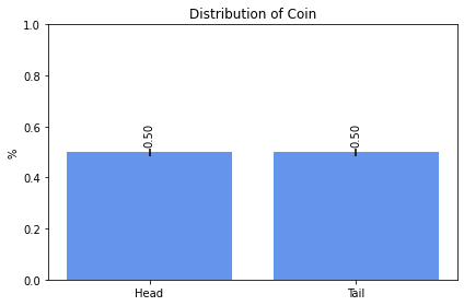
[42]:
fair_coin = Coin().set([.5] * 2)
fair_coin.plot(view=True)

biased_coin = Coin().set([.3, .7])
biased_coin.plot(view=True)
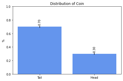
[43]:
biased_coin.p({'Head'})
[43]:
0.3
[44]:
biased_coin.mpe()
[44]:
(0.7, {'Tail'})
Random Variables
In pyjpt, random variables are instances of the jpt.variables.Variable class. jpt.Variable itself is abstract so it cannot be instantiated directly. There exist three subclasses
that implement the behavior of a variable of the respective type.
A variable is determined by its name and domain, which are passed as arguments in the variable object’s constructor. For instance, in order to instantiate two variables representing the result of the above coin tossing and dicing experiments, we create one integer and symbolic variable:
[45]:
from jpt.variables import SymbolicVariable, IntegerVariable

coin = SymbolicVariable('CoinToss', domain=Coin)
die = IntegerVariable('Dice', domain=Die)

coin, die
[45]:
(CoinToss[Coin], Dice[Die])
A variable object as such does not have much funcionality. Its main purpose is to bind a particular symbol in the domain of discource to the set of admissible values and to carry settings that are relevant for the learning and inference process.
Variable Assignments
The datastructure that describes questions and answers in JPTs are almost always jpt.variables.VariableAssignment. A VariableAssignment, as the name suggests, assigns instances of jpt.variables.Variable reference to values of their doamin. When creating queries and evidences for a JPT one is required to create VariableMaps or dict that map string to variable values. Variable values can be one of the following things
singular values: Singular values refer to numbers (ints or floats) for numeric variables or one element of a variables domain (most likely a string or int or float)
sets: For discrete variables a set should be a python set of elements of a variables domain. For numeric variables it can be either a ContinuousSet or RealSet. A ContinuousSet is a simple interval with lower and upper bound. A RealSet is a set of intervals in the same sense as for discrete variables. Those sets are interpreted as the statement: the value of variables x A or B or C for a something like
{"A", "B", "C"}