Learning of Joint Probability Distributions

This tutorial introduces the basics of learning joint probability distributions with jpt.trees.JPT. A JPT is trained on tabular data and learns a compact tree-structured representation of the joint distribution \(P(\mathcal{X})\) over all variables in the dataset.

We use the Iris dataset throughout this tutorial as a small, well-understood example with both numeric and symbolic variables.

Preparing the Data

JPTs consume plain pandas.DataFrame objects. We load the Iris dataset and add the class label as a string column so that pyjpt can recognise it as a symbolic variable.

import sklearn.datasets
import pandas as pd

dataset = sklearn.datasets.load_iris()
df = pd.DataFrame(columns=dataset.feature_names, data=dataset.data)

target = dataset.target.astype(object)
for idx, name in enumerate(dataset.target_names):
    target[target == idx] = name

df['plant'] = target
df.head()

	sepal length (cm)	sepal width (cm)	petal length (cm)	petal width (cm)	plant
0	5.1	3.5	1.4	0.2	setosa
1	4.9	3.0	1.4	0.2	setosa
2	4.7	3.2	1.3	0.2	setosa
3	4.6	3.1	1.5	0.2	setosa
4	5.0	3.6	1.4	0.2	setosa

Inferring Variables from a DataFrame

jpt.variables.infer_from_dataframe inspects the column types of a DataFrame and automatically creates the appropriate variable type for each column:

Column dtype	Variable type
float / int (numeric)	NumericVariable
object / category (strings)	SymbolicVariable
int (integer domain)	IntegerVariable

Variables can also be defined manually; see tutorial_variables for details.

from jpt.variables import infer_from_dataframe

variables = infer_from_dataframe(df)

for v in variables:
    print(v, type(v).__name__)

sepal length (cm)[SEPAL LENGTH (CM)_TYPE_N] NumericVariable
sepal width (cm)[SEPAL WIDTH (CM)_TYPE_N] NumericVariable
petal length (cm)[PETAL LENGTH (CM)_TYPE_N] NumericVariable
petal width (cm)[PETAL WIDTH (CM)_TYPE_N] NumericVariable
plant[PLANT_TYPE_S] SymbolicVariable

Creating and Fitting a JPT

A jpt.trees.JPT is created by passing the variable list to the constructor, and then trained by calling fit with the DataFrame.

The most important stopping criterion is min_samples_leaf, which sets the minimum number of training samples required in each leaf. Larger values produce smaller, less overfit trees; smaller values allow finer partitions at the cost of higher variance. Fractional values between 0 and 1 are interpreted as a fraction of the training set size.

from jpt.trees import JPT

model = JPT(variables, min_samples_leaf=0.1)
model.fit(df)
model

<JPT #innernodes = 6, #leaves = 7 (13 total)>

The printed tree shows the decision nodes and leaves that make up the partition. Each leaf stores an independent factorised distribution over all variables.

The number of parameters (i.e. the total size of all leaf distributions) can be queried directly:

print('Number of leaves:', len(model.leaves))
print('Number of parameters:', model.number_of_parameters())

Number of leaves: 7
Number of parameters: 206

Effect of Hyperparameters

Three hyperparameters control the tree structure:

Parameter	Effect
min_samples_leaf	Minimum samples per leaf (absolute or fraction)
max_depth	Maximum tree depth
min_impurity_improvement	Minimum impurity gain required to accept a split

The plot below shows how min_samples_leaf trades off model complexity (number of parameters) against data fit (log-likelihood on the training set).

import numpy as np
import matplotlib.pyplot as plt

min_samples_values = range(1, 51)
log_likelihoods = []
n_params = []

for msl in min_samples_values:
    m = JPT(variables, min_samples_leaf=msl)
    m.fit(df)
    ll = np.sum(np.log(m.likelihood(df)))
    log_likelihoods.append(ll)
    n_params.append(m.number_of_parameters())

fig, ax1 = plt.subplots()
ax2 = ax1.twinx()
ax1.plot(min_samples_values, log_likelihoods, color='tab:blue', label='log-likelihood')
ax2.plot(min_samples_values, n_params, color='tab:orange', label='# parameters')
ax1.set_xlabel('min_samples_leaf')
ax1.set_ylabel('log-likelihood', color='tab:blue')
ax2.set_ylabel('# parameters', color='tab:orange')
fig.legend(loc='upper right', bbox_to_anchor=(0.9, 0.85))
plt.title('Model complexity vs. data fit')
plt.tight_layout()
plt.show()

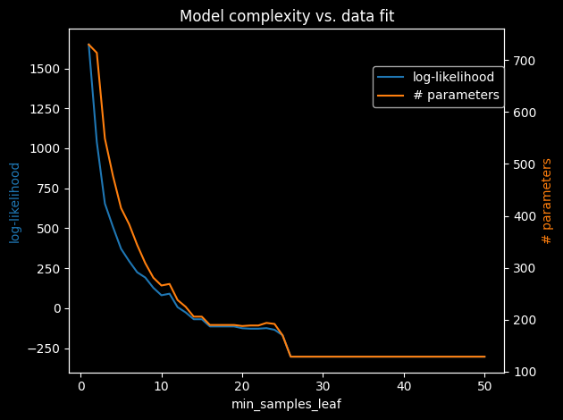
As expected, fewer samples per leaf means more leaves and more parameters, which increases the log-likelihood on the training data. In practice a value of 1–10 % of the dataset size is a good starting point.

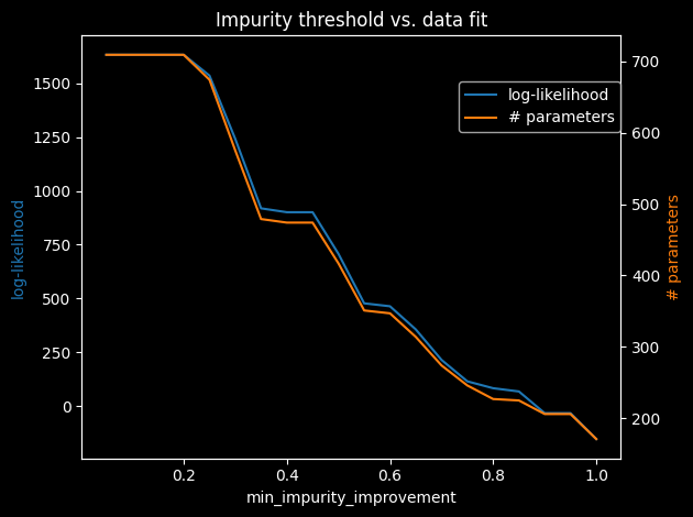
min_impurity_improvement enforces a minimum information-gain threshold before accepting a split and is a complementary regularisation knob:

thresholds = [i * 0.05 for i in range(1, 21)]
log_likelihoods_ii = []
n_params_ii = []

for thresh in thresholds:
    m = JPT(variables, min_impurity_improvement=thresh)
    m.fit(df)
    ll = np.sum(np.log(m.likelihood(df)))
    log_likelihoods_ii.append(ll)
    n_params_ii.append(m.number_of_parameters())

fig, ax1 = plt.subplots()
ax2 = ax1.twinx()
ax1.plot(thresholds, log_likelihoods_ii, color='tab:blue', label='log-likelihood')
ax2.plot(thresholds, n_params_ii, color='tab:orange', label='# parameters')
ax1.set_xlabel('min_impurity_improvement')
ax1.set_ylabel('log-likelihood', color='tab:blue')
ax2.set_ylabel('# parameters', color='tab:orange')
fig.legend(loc='upper right', bbox_to_anchor=(0.9, 0.85))
plt.title('Impurity threshold vs. data fit')
plt.tight_layout()
plt.show()

Generative vs. Discriminative Learning

By default a JPT learns the full joint distribution \(P(\mathcal{X})\) over all variables (generative mode). This is useful when any variable may play the role of a query or evidence variable at inference time.

When the task is specifically to predict a set of target variables \(Y\) from feature variables \(X = \mathcal{X} \setminus Y\), discriminative mode optimises the tree splits with respect to \(Y\) only. This concentrates the model’s representational capacity on predicting \(Y\) and typically yields better conditional predictions at the cost of a less accurate model of \(X\).

Discriminative mode is activated by passing a targets list to the constructor:

# Discriminative JPT: splits optimised for predicting 'plant'
varnames = {v.name: v for v in variables}

disc_model = JPT(
    variables,
    targets=[varnames['plant']],
    min_samples_leaf=0.1
)
disc_model.fit(df)
disc_model

<JPT #innernodes = 6, #leaves = 7 (13 total)>

Saving and Loading a Model

A trained model can be persisted to disk and reloaded later without re-running the training.

import tempfile, os

# Save
tmp = tempfile.mktemp(suffix='.json')
model.save(tmp)
print('Saved to', tmp)

# Load
loaded_model = JPT.load(tmp)
print('Loaded:', loaded_model)

os.remove(tmp)

Saved to /tmp/tmp0he4m98k.json
Loaded: JPT#innernodes = 6, #leaves = 7 (13 total)

The loaded model is identical to the original and can be used for inference without any further setup. See tutorial_reasoning for how to query a trained model.