Regression
This example will guide through a very noisy regression problem. First we have to create the regression data. The data will originate from the function \(x \cdot sin(x)\).
[5]:
import pandas as pd
import numpy as np
import logging

logging.getLogger("/jpt").setLevel(0)
def f(x):
    return x * np.sin(x)

def generate_data(func, x_lower, x_upper, n):
    '''
    Generate a ``DataFrame`` of ``n`` data samples with additive noise from the function ``func``.
    '''
    X = np.atleast_2d(np.random.uniform(-20, 0.0, size=int(n / 2))).T
    X = np.vstack((np.atleast_2d(np.random.uniform(0, 10.0, size=int(n / 2))).T, X))
    X = X.astype(np.float32)
    X = np.array(list(sorted(X)))

    # Observations
    y = func(X).ravel()

    # Add some noise
    dy = 1.5 + .5 * np.random.random(y.shape)
    y += np.random.normal(0, dy)
    y = y.astype(np.float32)

    return pd.DataFrame(data={'x': X.ravel(), 'y': y})

df = generate_data(f, -20, 10, 1000)
df
[5]:
| x | y | |
|---|---|---|
| 0 | -19.944950 | 18.102259 |
| 1 | -19.905794 | 16.782999 |
| 2 | -19.874876 | 16.939438 |
| 3 | -19.783342 | 12.793908 |
| 4 | -19.721155 | 18.745640 |
| ... | ... | ... |
| 995 | 9.941216 | -4.190035 |
| 996 | 9.944221 | -7.070674 |
| 997 | 9.953140 | -1.843960 |
| 998 | 9.957382 | -3.120459 |
| 999 | 9.965003 | -2.542398 |
1000 rows × 2 columns
Lets have a look at the data visually:
[6]:
import matplotlib
import matplotlib.pyplot as plt

plt.plot(df['x'].values, df['y'].values, '.', markersize=5, label='Training data')
plt.show()
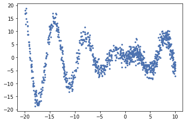
We can clearly see the original function, and we can observe that there is more variance towards higher x. In general, we don’t want a model that assumes independent noise, and we don’t want to specify much prior knowledge since it is only available rarely. Let’s specify a JPT that focuses on predicting y accurately.
[7]:
from jpt.variables import NumericVariable, VariableMap
from jpt.trees import JPT

# Construct the variables, soften up x via blur
varx = NumericVariable('x', blur=.05)
vary = NumericVariable('y')

# enable a focus on the parameters for y with the targets keyword
jpt = JPT(variables=[varx, vary], targets=[vary], min_samples_leaf=.01, min_impurity_improvement=0.01)

jpt.learn(data=df)
[7]:
JPT
<DecisionNode #0 x = [x < -15.944; -15.944 ≤ x]; parent-#: None; #children: 2>
    <DecisionNode #1 x = [x < -18.815; -18.815 ≤ x]; parent-#: 0; #children: 2>
        <DecisionNode #3 x = [x < -19.231; -19.231 ≤ x]; parent-#: 1; #children: 2>
            <Leaf #7; parent: <DecisionNode #3>>
            <Leaf #8; parent: <DecisionNode #3>>
        <DecisionNode #4 x = [x < -18.336; -18.336 ≤ x]; parent-#: 1; #children: 2>
            <Leaf #9; parent: <DecisionNode #4>>
            <DecisionNode #10 x = [x < -16.596; -16.596 ≤ x]; parent-#: 4; #children: 2>
                <DecisionNode #15 x = [x < -17.973; -17.973 ≤ x]; parent-#: 10; #children: 2>
                    <Leaf #23; parent: <DecisionNode #15>>
                    <DecisionNode #24 x = [x < -17.113; -17.113 ≤ x]; parent-#: 15; #children: 2>
                        <DecisionNode #33 x = [x < -17.637; -17.637 ≤ x]; parent-#: 24; #children: 2>
                            <Leaf #47; parent: <DecisionNode #33>>
                            <Leaf #48; parent: <DecisionNode #33>>
                        <Leaf #34; parent: <DecisionNode #24>>
                <Leaf #16; parent: <DecisionNode #10>>
    <DecisionNode #2 x = [x < -12.830; -12.830 ≤ x]; parent-#: 0; #children: 2>
        <DecisionNode #5 x = [x < -15.458; -15.458 ≤ x]; parent-#: 2; #children: 2>
            <Leaf #11; parent: <DecisionNode #5>>
            <DecisionNode #12 x = [x < -13.342; -13.342 ≤ x]; parent-#: 5; #children: 2>
                <DecisionNode #17 x = [x < -15.038; -15.038 ≤ x]; parent-#: 12; #children: 2>
                    <Leaf #25; parent: <DecisionNode #17>>
                    <DecisionNode #26 x = [x < -14.795; -14.795 ≤ x]; parent-#: 17; #children: 2>
                        <Leaf #35; parent: <DecisionNode #26>>
                        <DecisionNode #36 x = [x < -13.710; -13.710 ≤ x]; parent-#: 26; #children: 2>
                            <DecisionNode #49 x = [x < -14.202; -14.202 ≤ x]; parent-#: 36; #children: 2>
                                <Leaf #65; parent: <DecisionNode #49>>
                                <Leaf #66; parent: <DecisionNode #49>>
                            <Leaf #50; parent: <DecisionNode #36>>
                <Leaf #18; parent: <DecisionNode #12>>
        <DecisionNode #6 x = [x < -9.694; -9.694 ≤ x]; parent-#: 2; #children: 2>
            <DecisionNode #13 x = [x < -12.219; -12.219 ≤ x]; parent-#: 6; #children: 2>
                <Leaf #19; parent: <DecisionNode #13>>
                <DecisionNode #20 x = [x < -11.989; -11.989 ≤ x]; parent-#: 13; #children: 2>
                    <Leaf #27; parent: <DecisionNode #20>>
                    <DecisionNode #28 x = [x < -10.479; -10.479 ≤ x]; parent-#: 20; #children: 2>
                        <DecisionNode #37 x = [x < -11.625; -11.625 ≤ x]; parent-#: 28; #children: 2>
                            <Leaf #51; parent: <DecisionNode #37>>
                            <Leaf #52; parent: <DecisionNode #37>>
                        <Leaf #38; parent: <DecisionNode #28>>
            <DecisionNode #14 x = [x < 6.464; 6.464 ≤ x]; parent-#: 6; #children: 2>
                <DecisionNode #21 x = [x < -6.466; -6.466 ≤ x]; parent-#: 14; #children: 2>
                    <DecisionNode #29 x = [x < -9.112; -9.112 ≤ x]; parent-#: 21; #children: 2>
                        <Leaf #39; parent: <DecisionNode #29>>
                        <DecisionNode #40 x = [x < -7.079; -7.079 ≤ x]; parent-#: 29; #children: 2>
                            <DecisionNode #53 x = [x < -8.435; -8.435 ≤ x]; parent-#: 40; #children: 2>
                                <Leaf #67; parent: <DecisionNode #53>>
                                <DecisionNode #68 x = [x < -7.907; -7.907 ≤ x]; parent-#: 53; #children: 2>
                                    <Leaf #81; parent: <DecisionNode #68>>
                                    <Leaf #82; parent: <DecisionNode #68>>
                            <Leaf #54; parent: <DecisionNode #40>>
                    <DecisionNode #30 x = [x < 3.471; 3.471 ≤ x]; parent-#: 21; #children: 2>
                        <DecisionNode #41 x = [x < -3.720; -3.720 ≤ x]; parent-#: 30; #children: 2>
                            <DecisionNode #55 x = [x < -5.854; -5.854 ≤ x]; parent-#: 41; #children: 2>
                                <DecisionNode #69 x = [x < -6.143; -6.143 ≤ x]; parent-#: 55; #children: 2>
                                    <Leaf #83; parent: <DecisionNode #69>>
                                    <Leaf #84; parent: <DecisionNode #69>>
                                <DecisionNode #70 x = [x < -5.480; -5.480 ≤ x]; parent-#: 55; #children: 2>
                                    <Leaf #85; parent: <DecisionNode #70>>
                                    <DecisionNode #86 x = [x < -4.448; -4.448 ≤ x]; parent-#: 70; #children: 2>
                                        <DecisionNode #95 x = [x < -5.187; -5.187 ≤ x]; parent-#: 86; #children: 2>
                                            <Leaf #103; parent: <DecisionNode #95>>
                                            <Leaf #104; parent: <DecisionNode #95>>
                                        <Leaf #96; parent: <DecisionNode #86>>
                            <DecisionNode #56 x = [x < 2.985; 2.985 ≤ x]; parent-#: 41; #children: 2>
                                <DecisionNode #71 x = [x < 0.987; 0.987 ≤ x]; parent-#: 56; #children: 2>
                                    <DecisionNode #87 x = [x < -0.231; -0.231 ≤ x]; parent-#: 71; #children: 2>
                                        <DecisionNode #97 x = [x < -2.979; -2.979 ≤ x]; parent-#: 87; #children: 2>
                                            <Leaf #105; parent: <DecisionNode #97>>
                                            <DecisionNode #106 x = [x < -0.756; -0.756 ≤ x]; parent-#: 97; #children: 2>
                                                <DecisionNode #113 x = [x < -2.410; -2.410 ≤ x]; parent-#: 106; #children: 2>
                                                    <Leaf #119; parent: <DecisionNode #113>>
                                                    <DecisionNode #120 x = [x < -1.058; -1.058 ≤ x]; parent-#: 113; #children: 2>
                                                        <Leaf #123; parent: <DecisionNode #120>>
                                                        <Leaf #124; parent: <DecisionNode #120>>
                                                <Leaf #114; parent: <DecisionNode #106>>
                                        <DecisionNode #98 x = [x < 0.549; 0.549 ≤ x]; parent-#: 87; #children: 2>
                                            <DecisionNode #107 x = [x < 0.300; 0.300 ≤ x]; parent-#: 98; #children: 2>
                                                <DecisionNode #115 x = [x < 0.106; 0.106 ≤ x]; parent-#: 107; #children: 2>
                                                    <Leaf #121; parent: <DecisionNode #115>>
                                                    <Leaf #122; parent: <DecisionNode #115>>
                                                <Leaf #116; parent: <DecisionNode #107>>
                                            <DecisionNode #108 x = [x < 0.851; 0.851 ≤ x]; parent-#: 98; #children: 2>
                                                <Leaf #117; parent: <DecisionNode #108>>
                                                <Leaf #118; parent: <DecisionNode #108>>
                                    <DecisionNode #88 x = [x < 2.461; 2.461 ≤ x]; parent-#: 71; #children: 2>
                                        <DecisionNode #99 x = [x < 2.127; 2.127 ≤ x]; parent-#: 88; #children: 2>
                                            <Leaf #109; parent: <DecisionNode #99>>
                                            <Leaf #110; parent: <DecisionNode #99>>
                                        <DecisionNode #100 x = [x < 2.797; 2.797 ≤ x]; parent-#: 88; #children: 2>
                                            <Leaf #111; parent: <DecisionNode #100>>
                                            <Leaf #112; parent: <DecisionNode #100>>
                                <DecisionNode #72 x = [x < 3.257; 3.257 ≤ x]; parent-#: 56; #children: 2>
                                    <Leaf #89; parent: <DecisionNode #72>>
                                    <Leaf #90; parent: <DecisionNode #72>>
                        <DecisionNode #42 x = [x < 5.913; 5.913 ≤ x]; parent-#: 30; #children: 2>
                            <DecisionNode #57 x = [x < 3.791; 3.791 ≤ x]; parent-#: 42; #children: 2>
                                <Leaf #73; parent: <DecisionNode #57>>
                                <DecisionNode #74 x = [x < 5.714; 5.714 ≤ x]; parent-#: 57; #children: 2>
                                    <DecisionNode #91 x = [x < 4.162; 4.162 ≤ x]; parent-#: 74; #children: 2>
                                        <Leaf #101; parent: <DecisionNode #91>>
                                        <Leaf #102; parent: <DecisionNode #91>>
                                    <Leaf #92; parent: <DecisionNode #74>>
                            <DecisionNode #58 x = [x < 6.304; 6.304 ≤ x]; parent-#: 42; #children: 2>
                                <Leaf #75; parent: <DecisionNode #58>>
                                <Leaf #76; parent: <DecisionNode #58>>
                <DecisionNode #22 x = [x < 9.243; 9.243 ≤ x]; parent-#: 14; #children: 2>
                    <DecisionNode #31 x = [x < 7.011; 7.011 ≤ x]; parent-#: 22; #children: 2>
                        <DecisionNode #43 x = [x < 6.837; 6.837 ≤ x]; parent-#: 31; #children: 2>
                            <Leaf #59; parent: <DecisionNode #43>>
                            <Leaf #60; parent: <DecisionNode #43>>
                        <DecisionNode #44 x = [x < 8.834; 8.834 ≤ x]; parent-#: 31; #children: 2>
                            <DecisionNode #61 x = [x < 8.552; 8.552 ≤ x]; parent-#: 44; #children: 2>
                                <DecisionNode #77 x = [x < 7.556; 7.556 ≤ x]; parent-#: 61; #children: 2>
                                    <Leaf #93; parent: <DecisionNode #77>>
                                    <Leaf #94; parent: <DecisionNode #77>>
                                <Leaf #78; parent: <DecisionNode #61>>
                            <DecisionNode #62 x = [x < 8.957; 8.957 ≤ x]; parent-#: 44; #children: 2>
                                <Leaf #79; parent: <DecisionNode #62>>
                                <Leaf #80; parent: <DecisionNode #62>>
                    <DecisionNode #32 x = [x < 9.496; 9.496 ≤ x]; parent-#: 22; #children: 2>
                        <Leaf #45; parent: <DecisionNode #32>>
                        <DecisionNode #46 x = [x < 9.763; 9.763 ≤ x]; parent-#: 32; #children: 2>
                            <Leaf #63; parent: <DecisionNode #46>>
                            <Leaf #64; parent: <DecisionNode #46>>

JPT stats: #innernodes = 62, #leaves = 63 (125 total)
Since the data is 2D we can get a visual representation of the predictions of the JPT. Let’s plot the predictions and get an idea of the distribution. We will plot the expectation of y for every datapoint on the x-axis and confidence intervals that explain 95% of the variance.
[8]:
# Mesh the input space for evaluations of the real function,
# the prediction and its MSE
xx = np.atleast_2d(np.linspace(-20, 15, 500)).astype(np.float32).T

# Apply the JPT model
confidence = .95
conf_level = 0.95
my_predictions = [jpt.posterior([vary], evidence={varx: x_}, fail_on_unsatisfiability=False) for x_ in xx.ravel()]
y_pred_ = [(p[vary].expectation() if p is not None else None) for p in my_predictions]
y_lower_ = [(p[vary].ppf.eval((1 - conf_level) / 2) if p is not None else None) for p in my_predictions]
y_upper_ = [(p[vary].ppf.eval(1 - (1 - conf_level) / 2) if p is not None else None) for p in my_predictions]

# posterior = jpt.posterior([varx], {vary: 0})

# Plot the function, the prediction and the 90% confidence interval based on the MSE
plt.plot(xx, f(xx), color='black', linestyle=':', linewidth='2', label=r'$f(x) = x\,\sin(x)$')
plt.plot(df['x'].values, df['y'].values, '.', color='gray', markersize=5, label='Training data')
plt.plot(xx, y_pred_, 'm-', label='JPT Prediction', linewidth=2)
plt.plot(xx, y_lower_, 'y--', label='%.1f%% Confidence bands' % (confidence * 100))
plt.plot(xx, y_upper_, 'y--')
# plt.plot(xx, np.asarray(posterior.distributions[varx].pdf.multi_eval(xx.ravel().astype(np.float64))),
#          label='Posterior')
plt.plot(xx, np.array([jpt.pdf(VariableMap([(varx, x_), (vary, 0)])) for x_ in xx.ravel().astype(np.float64)]),
         label='Posterior')

plt.xlabel('$x$')
plt.ylabel('$f(x)$')
plt.ylim(-10, 20)
plt.xlim(-25, 15)
plt.legend(loc='upper left')
plt.title(r'2D Regression Example ($\vartheta=%.2f\%%$)' % (confidence * 100))
plt.grid()

plt.show()

As we can see the expectations and variances predicted by the JPT characterize this dataset well and the variance even adjusts to the different x values. Impressive!