Reasoning about Joint Probability Distributions

This tutorial walks through the inference capabilities of jpt.trees.JPT. We cover every supported query type:

Query	Method	Returns
Marginal \(P(\mathcal{E}=e)\)	infer	float
Conditional \(P(Q \mid E)\)	infer	float
Posterior distributions \(P(Q \mid E)\)	posterior	VariableMap of distributions
Expected values \(\mathbb{E}[Q \mid E]\)	expectation	VariableMap of scalars
Most probable explanation (MPE)	mpe	assignment + likelihood
\(k\) most probable explanations	kmpe	iterator of assignments

We first train a model on the Iris dataset (the same setup as in tutorial_learning).

import sklearn.datasets
import pandas as pd
from jpt.variables import infer_from_dataframe
from jpt.trees import JPT

dataset = sklearn.datasets.load_iris()
df = pd.DataFrame(columns=dataset.feature_names, data=dataset.data)

target = dataset.target.astype(object)
for idx, name in enumerate(dataset.target_names):
    target[target == idx] = name

df['plant'] = target

variables = infer_from_dataframe(df)
varnames = {v.name: v for v in variables}

model = JPT(variables, min_samples_leaf=0.1)
model.fit(df)
model

<JPT #innernodes = 6, #leaves = 7 (13 total)>

Marginal Queries

A marginal query computes the probability of a partial state \(P(\mathcal{E} = e)\) by integrating out all unassigned variables. In pyjpt this is expressed as a call to infer with a query but no evidence.

The query is a plain Python dict mapping variable names (or variable objects) to values or ranges. Ranges for numeric variables are given as two-element lists [lower, upper].

# P(plant = 'setosa')
p_setosa = model.infer(query={'plant': 'setosa'})
print(f'P(plant=setosa) = {p_setosa:.4f}')

# P(sepal length in [5, 6])
p_sepal = model.infer(query={'sepal length (cm)': [5., 6.]})
print(f'P(sepal length in [5,6]) = {p_sepal:.4f}')

# Joint marginal: P(plant in {setosa, versicolor} AND sepal length in [5, 6])
p_joint = model.infer(
    query={
        'plant': {'setosa', 'versicolor'},
        'sepal length (cm)': [5., 6.]
    }
)
print(f'P(plant in {{setosa,versicolor}}, sepal in [5,6]) = {p_joint:.4f}')

P(plant=setosa) = 0.3333
P(sepal length in [5,6]) = 0.3861
P(plant in {setosa,versicolor}, sepal in [5,6]) = 0.3310

Conditional Queries

A conditional query computes \(P(Q \mid E) = P(Q, E) / P(E)\). The query argument specifies \(Q\) and the evidence argument specifies \(E\). The method returns a scalar probability.

# P(plant = 'virginica' | sepal length in [6, 7])
p_cond = model.infer(
    query={'plant': 'virginica'},
    evidence={'sepal length (cm)': [6., 7.]}
)
print(f'P(plant=virginica | sepal in [6,7]) = {p_cond:.4f}')

# P(petal length > 4 | plant = 'versicolor')
p_petal = model.infer(
    query={'petal length (cm)': [4., float('inf')]},
    evidence={'plant': 'versicolor'}
)
print(f'P(petal length > 4 | plant=versicolor) = {p_petal:.4f}')

P(plant=virginica | sepal in [6,7]) = 0.5918
P(petal length > 4 | plant=versicolor) = 0.6864

When the evidence has zero probability (unsatisfiable), infer raises an exception by default. Pass fail_on_unsatisfiability=False to get None instead:

result = model.infer(
    query={'plant': 'setosa'},
    evidence={'plant': 'virginica'},
    fail_on_unsatisfiability=False
)
print('Result for contradictory evidence:', result)

Result for contradictory evidence: 0.0

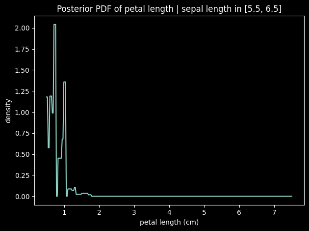
Posterior Distributions

While infer collapses the answer to a single number, posterior returns the full posterior distribution over each query variable given the evidence. The result is a VariableMap mapping each variable to its posterior distribution object.

For numeric variables the posterior is a Numeric distribution; its pdf and cdf attributes are callable functions over the real line.

For symbolic variables the posterior is a Multinomial distribution; its probabilities array is indexed in the same order as variable.domain.

import numpy as np
import matplotlib.pyplot as plt

post = model.posterior(
    variables=[varnames['petal length (cm)'], varnames['plant']],
    evidence={'sepal length (cm)': [5.5, 6.5]}
)

# --- Numeric posterior: plot the PDF ---
petal_dist = post[varnames['petal length (cm)']]
x = np.linspace(0.5, 7.5, 300)
y = [petal_dist.pdf(xi) for xi in x]

plt.figure()
plt.plot(x, y)
plt.xlabel('petal length (cm)')
plt.ylabel('density')
plt.title('Posterior PDF of petal length | sepal length in [5.5, 6.5]')
plt.tight_layout()
plt.show()

# --- Symbolic posterior: bar chart ---
plant_dist = post[varnames['plant']]
labels = list(varnames['plant'].domain)
probs = [plant_dist.p(label) for label in labels]

plt.figure()
plt.bar(labels, probs)
plt.ylabel('probability')
plt.title('Posterior P(plant | sepal length in [5.5, 6.5])')
plt.tight_layout()
plt.show()

---------------------------------------------------------------------------
TypeError                                 Traceback (most recent call last)
Cell In[5], line 24
     22 # --- Symbolic posterior: bar chart ---
     23 plant_dist = post[varnames['plant']]
---> 24 labels = list(varnames['plant'].domain)
     25 probs = [plant_dist.p(label) for label in labels]
     27 plt.figure()

TypeError: 'type' object is not iterable

Note that the posterior variables are returned independently: the VariableMap does not encode the joint distribution over the query variables, only the marginal of each. If you need the full conditional joint distribution, use conditional_jpt.

Expectations

expectation computes \(\mathbb{E}[Q_i \mid E]\) for each variable in a query set and returns a VariableMap of scalar values.

For symbolic variables the expectation is not defined; those variables are silently skipped.

numeric_vars = [
    varnames['sepal width (cm)'],
    varnames['petal length (cm)'],
    varnames['petal width (cm)']
]

exp = model.expectation(
    variables=numeric_vars,
    evidence={'plant': 'versicolor'}
)

for var, value in exp.items():
    print(f'E[{var.name} | plant=versicolor] = {value:.4f}')

E[sepal width (cm) | plant=versicolor] = 2.7411
E[petal length (cm) | plant=versicolor] = 4.1313
E[petal width (cm) | plant=versicolor] = nan

Most Probable Explanation (MPE)

The most probable explanation query answers \(\operatorname{argmax}_{Q} P(Q \mid E)\): given evidence \(E\), find the assignment of unobserved variables that jointly maximises the probability.

mpe returns a tuple of (assignments, likelihood). assignments is a list of LabelAssignment objects — multiple assignments may be returned when several leaves tie for the maximum. The likelihood is the joint probability density/mass of the best assignment.

assignments, likelihood = model.mpe(
    evidence={'plant': 'virginica'}
)

print(f'Likelihood of best explanation: {likelihood:.6f}')
for i, assignment in enumerate(assignments):
    print(f'  Assignment {i}: {assignment}')

Likelihood of best explanation: 7.072741
  Assignment 0: <LabelAssignment {sepal length (cm): <ContinuousSet=[6.200,6.400)>, sepal width (cm): <ContinuousSet=[3.000,3.100)>, petal length (cm): <ContinuousSet=[5.500,5.600)>, petal width (cm): <ContinuousSet=[2.200,2.300)>, plant: {np.str_('virginica')}}>

k Most Probable Explanations (k-MPE)

kmpe generalises MPE to return an iterator that yields the \(k\) best explanations in descending order of likelihood. This is useful when the single best assignment is not sufficient, e.g. to present a ranked list of hypotheses.

Set k=0 to retrieve all explanations (bounded by the number of leaves).

k = 3

print(f'Top-{k} explanations given plant=versicolor:\n')
for rank, (assignment, likelihood) in enumerate(
        model.kmpe(evidence={'plant': 'versicolor'}, k=k),
        start=1
):
    print(f'  Rank {rank}  (likelihood={likelihood:.6f})')
    print(f'    {assignment}\n')

Top-3 explanations given plant=versicolor:

  Rank 1  (likelihood=4.204493)
    <LabelAssignment {plant: {np.str_('versicolor')}, petal width (cm): <ContinuousSet=[1.400,1.500)>, petal length (cm): <ContinuousSet=[4.300,4.500)>, sepal width (cm): <ContinuousSet=[2.800,2.900)>, sepal length (cm): <ContinuousSet=[6.000,6.100)>}>

  Rank 2  (likelihood=3.822266)
    <LabelAssignment {plant: {np.str_('versicolor')}, petal width (cm): <ContinuousSet=[1.400,1.500)>, petal length (cm): <ContinuousSet=[4.600,4.700)>, sepal width (cm): <ContinuousSet=[2.800,2.900)>, sepal length (cm): <ContinuousSet=[6.000,6.100)>}>

  Rank 3  (likelihood=3.503744)
    <LabelAssignment {plant: {np.str_('versicolor')}, petal width (cm): <ContinuousSet=[1.400,1.500)>, petal length (cm): <ContinuousSet=[4.300,4.500)>, sepal width (cm): <ContinuousSet=[2.800,2.900)>, sepal length (cm): <ContinuousSet=[6.100,6.300)>}>

Using bind to Construct Queries

All inference methods accept raw Python dict objects, but bind can be used to construct a validated LabelAssignment explicitly. This is useful for reusing and inspecting queries, or when building queries programmatically.

See important_datastructures for a full treatment of LabelAssignment and the underlying set types.

query = model.bind({
    'plant': {'setosa', 'versicolor'},
    'sepal length (cm)': [5., 6.]
})
evidence = model.bind({'petal width (cm)': [0., 1.]})

print('Query:   ', query)
print('Evidence:', evidence)

p = model.infer(query=query, evidence=evidence)
print(f'\nP(query | evidence) = {p:.4f}')